

Effective gross income (EGI) is the total revenue a property is realistically expected to collect over a defined period, adjusted for vacancy and credit loss.
The standard formula is:
EGI = Potential Gross Income (PGI) − Vacancy Loss − Credit Loss + Other Income.
In everyday underwriting, vacancy and credit loss are typically combined into a single blended percentage deduction, commonly 5 to 10 percent for a stabilized asset.
Institutional practice (that we apply in our approaches) separates them and constructs each from specific data rather than a market average, because the number that lands in a pro forma determines how much income the lender assumes the property will generate. Both lenders and experienced LPs will ask exactly how it was derived.
From Potential Gross Income to EGI: The Full Waterfall
The standard shorthand collapses several real income adjustments into a single deduction line. Institutional underwriters surface each as a separate step, for good reason. Let’s break it down.
| Step | Line Item | What It Represents |
| 1 | Gross Potential Rent (GPR) | 100% of units occupied at 100% market rent – the theoretical maximum |
| 2 | Less: Loss to Lease | Gap between in-place contract rents and current market rents on occupied units |
| 3 | Equals: In-Place Rental Revenue | What the current rent roll actually generates at current lease rates |
| 4 | Less: Concessions | Move-in incentives, free rent periods, and other rent abatements |
| 5 | Less: Credit Loss (Bad Debt) | Rent billed but never collected. This is the economic cost of tenant non-payment |
| 6 | Less: Model Units | Units held offline for leasing and marketing purposes |
| 7 | Less: General Vacancy | Remaining unoccupied units not already captured in the steps above |
| 8 | Equals: Net Rental Income | Rental revenue after all deductions |
| 9 | Plus: Other Income | Parking, laundry, pet rent, storage fees, utility reimbursements |
| 10 | Equals: Effective Gross Income (EGI) | The realistic, collectable total property revenue |
In Real Estate Financial Modeling, introductory analysis and first-pass underwriting often compress steps 2 through 7 into a single vacancy and credit loss assumption applied to GPR. That approach is not necessarily wrong. But the key question is whether that level of simplification fits the asset and whether a lender or equity partner will expect a more detailed breakdown.
In one of the cases with mixed-use property in Texas, BlueStart team had to model and project precise vacancy per each unit.
Loss to lease and model units are the two items most commonly omitted from simplified EGI presentations, and both carry real financial consequences.
Loss to lease arises when a value-add or repositioning deal involves units currently leased below market rent. If a 100-unit building is fully occupied at $1,400 per month while market rents run $1,600, the rent roll generates $1.4M annually while GPR reflects $1.6M.
That $200,000 gap is loss to lease. The investment thesis depends on recovering it, but it is absent from current income until leases turn over at market rates.
Model units are a different animal. They are typically two to four units in a larger multifamily property held offline, furnished, and shown to prospective tenants. They generate no rent, yet they reduce the unit count available for occupancy.
At $1,500 per month per unit, two model units represent $36,000 in annual revenue the property structurally cannot collect. If model units are included in the full 100-unit count, the vacancy assumption is being applied to an overstated rental base.
How to Build a Vacancy Assumption
A flat vacancy percentage is common practice and defensible for a first-pass screen on a stabilized, homogeneous CRE asset. Its limitation is that it averages across a property’s entire unit mix, lease expiration schedule, and tenant quality as if those factors were uniform. But this rarely happens in the real world.
Institutional underwriting tools, most prominently ARGUS Enterprise, model vacancy at the unit or lease level through what the software calls Market Leasing Assumptions.
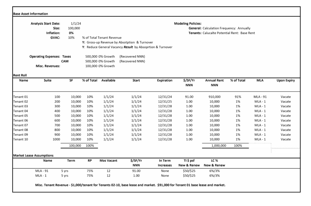
Each lease is individually modeled with its own renewal probability, an estimated downtime between move-out and the next lease signing, and a concession load. The resulting vacancy exposure is the aggregate of those individual unit outcomes, not a property-wide average applied from the top down.
ARGUS further distinguishes Absorption and Turnover Vacancy (vacancy periods triggered by individual lease events) from General Vacancy (a residual market-level adjustment). When an analyst applying both without care, it creates a real risk of double-counting vacancy loss. At BlueStar we typically see and flag these types of errors.
The flat-percentage approach holds up well when leases are naturally staggered across the calendar year, the tenant base is relatively homogeneous in payment behavior, and the property is genuinely stabilized. It starts to mislead in 3 specific situations.
| Situation | Why the Flat Assumption Breaks Down |
| Lease expiration concentration | Several large leases rolling in the same window creates outsized short-term vacancy exposure that an annual average obscures |
| Value-add repositioning | A deliberate re-tenanting plan means vacancy is not random but programmatic and needs to be modeled sequentially |
| Office or retail with anchor tenants | A single tenant occupying 30 percent or more of the building means one lease decision swings the whole property; a flat percentage offers almost no analytical value in this case |
One practitioner’s account captures the risk precisely. A team underwrote a Class C multifamily deal at a standard 5 percent economic vacancy assumption, reasonable by any general benchmark, and later found actual losses running two to three times that figure.
The problem was not that 5 percent is wrong in the abstract. It was that collecting rent from that specific tenant base, in that specific submarket, takes materially more time and effort than a flat assumption can reflect. The assumption was appropriate for the asset class in general; it was not appropriate for that asset.
How to Build a Credit Loss Assumption
Credit loss, sometimes called bad debt, is the portion of billed rent that tenants do not pay.
It is distinct from vacancy: a vacant unit produces no rent, while a credit loss is rent that was owed but not collected from an occupied unit. The two are frequently collapsed into a single blended deduction, which is workable as a shorthand but obscures a real methodological question: how was the credit loss component actually sized?
Rigorous underwriting builds credit loss from layered data rather than a market average.
Step 1: National historical baseline. Credit loss data gathered across full market cycles, including the worst historical periods, establishes both a typical level and a realistic worst-case range.
Step 2: Regional and market-level narrowing. National figures are refined by regional economic conditions. A national average applied to a high-turnover submarket consistently understates the real exposure.
Step 3: Tenant-quality adjustment. Income-to-rent ratio is a trackable, meaningful signal. When area median income is strong relative to asking rents, credit loss tends to run lower. In lower-income submarkets where rent consumes a higher share of household income, it tends to run meaningfully higher.
Step 4: Conservative bias. Underwriters often assume credit loss will run above the historical average rather than rely on a best-case scenario. In our practice, the estimate is considered as a conservative baseline, not an upper limit.
Where do current benchmarks land?
For multifamily, a reasonable first-pass credit loss assumption is typically around 1 to 2 percent of gross income, adjusted for tenant quality and submarket conditions. Some experienced operators use a combined vacancy and credit loss floor of about 6.5 percent as a conservative baseline, even when recent collections look stronger.
By comparison, conventional underwriting has often used roughly 50 basis points for bad debt at stabilization. Practitioners frequently view that as too low because it can understate the full cost of tenant default, including collection and legal expenses.
The hidden bad debt issue deserves a closer look. A seller or broker may report a trailing bad debt figure that appears low, even when collection problems are more significant. In some cases, units tied to chronic nonpayment are recorded as vacant rather than as bad debt.
The loss still exists, but it shows up under vacancy instead, making the stated bad debt rate look better than the property’s actual revenue performance.
Standard vs. Institutional EGI: A Side-by-Side Example
To make the methodology concrete, here is the same 80-unit multifamily property modeled both ways. Monthly market rent is $1,500 per unit; in-place contract rents average $1,420 per unit.
| Line Item | Simple Model | Institutional Model |
| Gross Potential Rent (GPR) | $1,440,000 | $1,440,000 |
| Loss to Lease | Not modeled | ($64,000) |
| In-Place Rental Revenue | $1,440,000 | $1,376,000 |
| Model Units (2 units) | Not modeled | ($36,000) |
| Concessions | Not modeled | ($14,400) |
| Vacancy Loss (6.5% / per-unit) | ($93,600) | ($72,000) |
| Credit Loss (1.5%) | Included above | ($21,600) |
| Net Rental Income | $1,346,400 | $1,232,000 |
| Other Income (parking, laundry) | $24,000 | $24,000 |
| Effective Gross Income | $1,370,400 | $1,256,000 |
The two approaches produce a $114,000 spread on annual EGI of more than 8%. That gap flows directly into NOI, and at a 5.5 percent exit cap rate, a $114,000 difference in stabilized NOI translates to roughly $2 million in projected property value at sale.
The rigorous approach may not always produce a dramatically different number. What it does produce is a defensible, auditable trail showing exactly how the figure was built, which is what a construction lender or sophisticated LP will ask to see before committing capital.
Five Mistakes That Understate Effective Gross Income
Let’s look of the typical mistakes. Each can be fixed using the methodology that we described here.
| Mistake | What Gets Missed | Why It Matters |
| Accepting the seller’s stated bad debt figure without scrutiny | Properties with chronic collection problems may record units as vacant rather than as uncollected, suppressing the apparent bad debt rate while the real economic loss is buried in vacancy | Due diligence should pull actual rent rolls and collections history, not rely on the stated figure |
| Applying a Class A vacancy benchmark to a Class C asset | The 5 percent convention is calibrated for quality tenant bases; lower-income properties consistently experience higher collection friction and longer turnover periods | The resulting effective gross income is overstated, and the pro forma will not survive actual operations |
| Omitting loss to lease on a value-add deal | The investment thesis depends on rent growth that has not yet occurred; ignoring the current gap makes Year 1 EGI appear stronger than it is | Overstates current-year income and may distort yield-on-cost calculations used to evaluate entry pricing |
| Failing to exclude model units from the rentable denominator | Two or three offline units represent $30,000 to $50,000 or more in annual uncollectable revenue at typical rents | A vacancy percentage applied to the total unit count includes units that structurally cannot generate rent |
| Double-counting vacancy by applying both per-unit ARGUS-style modeling and a separate general vacancy overlay | The two deductions are designed to capture different exposures; applied together without separation, they overlap and artificially suppress modeled EGI | The error typically surfaces during lender underwriting review, at a stage where revising the model can delay or complicate the financing process |
How BlueStar Consulting Builds EGI
BlueStar Consulting constructs effective gross income as part of its financial modeling, underwriting, and feasibility analysis work. The approach starts with the full revenue waterfall rather than a single blended percentage.
Vacancy and credit loss are modeled separately using asset-level and submarket data, with both assumptions clearly documented for lender and LP review.
For investors reviewing a sponsor’s pro forma or developers building one for the first time, BlueStar Consulting’s real estate financial modeling guide and real estate underwriting guide walk through how each line above the NOI is constructed and what questions to ask about every assumption before capital changes hands.
Frequently Asked Questions
What is the difference between effective gross income and net operating income?
Effective gross income is the revenue line. Net operating income (NOI) is what remains after operating expenses are subtracted from EGI. The relationship is straightforward: NOI = EGI minus Operating Expenses. EGI captures all the revenue adjustments (vacancy, credit loss, other income), while NOI is the first number that directly reflects the property’s operating profitability.
A detailed walkthrough of how NOI is built from EGI is covered in BlueStar Consulting’s article on NOI in real estate.
Does effective gross income include security deposits?
No. Security deposits are a liability on the property owner’s balance sheet, held on behalf of the tenant and either returned at lease expiration or applied against unpaid rent and damages. Including them in EGI overstates revenue and misrepresents the property’s cash flow. They do not appear anywhere in the EGI waterfall.
Is gross operating income the same thing as effective gross income?
The two terms are often used interchangeably, but different sources define them with subtle variation. In many institutional pro formas, gross operating income (GOI) is a direct synonym for EGI: total collectable revenue after vacancy and credit loss. In some models, EGI refers specifically to the rental revenue line, with other income added afterward to reach GOI. Clarifying which definition a given model is using is always worth confirming before comparing figures across sources.
Can effective gross income be higher than potential gross income?
In theory, yes. If the other income component (parking, storage, laundry, fee income) is large enough relative to vacancy and credit loss, EGI could technically exceed the gross potential rent from leasing alone. In practice, this is uncommon for most residential or standard commercial properties. It appears more often in assets with substantial ancillary revenue streams, such as a mixed-use building with strong retail or a property with a meaningful parking operation.
Is loss to lease the same thing as vacancy loss?
No, and the distinction matters. Loss to lease is the gap between what occupied units are currently generating at in-place contract rents and what those same units would generate if leased today at current market rents. The units are occupied and producing income, just less than full market rent. Vacancy loss, by contrast, reflects units that are unoccupied and generating no rent at all. Both reduce effective gross income, but from entirely different starting conditions, and each is sized using different inputs.
How often should vacancy and credit loss assumptions be updated during a hold period?
At minimum, annually as part of a budget and reforecast cycle. Any time the tenant base changes materially – a major move-out, an influx of renewals at below-market rents, or a shift in the submarket’s credit profile – the assumptions should be revisited before that change flows uncorrected into the DCF model. Stale assumptions applied to a property that has operationally shifted are one of the more reliable sources of divergence between projected and actual NOI in the later years of a hold.