

DCF sensitivity analysis in real estate re-runs a discounted cash flow model while one or two assumptions change, then records how IRR, equity multiple, or value responds. In commercial real estate, the assumptions that usually move a levered return most are rent growth, exit cap rate, vacancy, interest rate, and operating expense growth. The output shows which assumption the deal depends on, and how far each can miss before returns fall below the target.
In the worked example below, a 56 bps rise in the exit cap rate removes an 8% preferred return while the lender’s DSCR stays at 1.67x. Both results come from the same cash flows, read by two different audiences. The analysis applies to analysts and sponsors preparing a capital package, as well as investors reviewing one.
DCF sensitivity analysis belongs in underwriting, not after it. The pro forma is the base case, the financial model is the engine that lets assumptions change, and the sensitivity analysis is the output layer.
Four Tools, Four Questions
Each tool answers a different question. A complete analysis uses all four.
| Tool | Question it answers | Output | Covered in |
| One-way test with ranking (tornado) | Which assumption moves the return most? | Ranked table | Step 4 |
| Two-way table | How do the top two assumptions interact? | Grid of IRR or equity multiple | Step 5 |
| Breakeven | How wrong can an assumption be before the target fails? | A threshold value | Step 6 |
| Combined case | What happens if variables move together? | IRR, equity multiple, DSCR | Step 7 |
The first tool ranks the variables. The second shows how the top two interact. The third answers the question capital partners ask first: how far is the base case from the threshold. The fourth tests what happens when variables move together, which is how market disruptions typically arrive.
The Deal Used in Every Example
All figures in this article are illustrative examples computed for this brief. They are not market data and do not represent a specific property.
Table A. Deal assumptions
| Assumption | Value | Note |
| Property | 120-unit multifamily | Garden style, stabilized |
| Purchase price | $24,000,000 | $200,000 per unit. Closing costs 1.5%. |
| In-place rent | $1,650/unit/month | Rent growth 3.0% per year |
| Other income | $900/unit/year | Grows 3.0% per year |
| Vacancy and credit loss | 7.0% | Flat across the hold |
| Operating expenses | $5,900/unit/year | Grows 3.0% per year |
| Capex reserve | $300/unit/year | Held flat |
| Debt | $15,600,000 (65% LTV) | Interest only at 6.00% |
| Hold and exit | 5 years; exit cap rate 7.00% | Sale cost 2.0%. Exit value from year-6 NOI. |
| Preferred return (hurdle) | 8.0% | Used to shade the grid and set breakevens |
The model excludes taxes, amortization, fees, and promote. Exit value equals year-6 net operating income (NOI) divided by the exit cap rate. These simplifications make the sensitivity results easier to trace through each step.
Table B. Base case results
| Metric | Result | Note |
| Year-1 NOI | $1,609,680 | Going-in cap rate 6.71% |
| Year-6 NOI (exit basis) | $1,866,060 | Exit value $26,658,004 |
| Equity invested | $8,760,000 | Price plus closing costs minus loan |
| Levered IRR | 11.49% | Equity multiple 1.62x |
| Unlevered IRR | 8.07% | Equity multiple 1.42x |
| Year-1 DSCR | 1.72x | Debt yield 10.3% |
The base case sits at 11.49% levered IRR against an 8.0% preferred return. Every sensitivity result below is measured from this starting point.
How to Run a Sensitivity Analysis on a Real Estate DCF in 7 Steps
Step 1. Fix the Base Case and the Output Metrics
Confirm in-place rents, a market-supported growth rate, and a defensible exit cap rate before running any sensitivity test. If the base case is optimistic, every result in the grid starts too high.
Choose three output metrics: levered IRR (internal rate of return), equity multiple, and year-1 debt service coverage ratio (DSCR). Add the investor hurdle, here 8.0%. These three metrics let the analysis speak to two audiences at once: equity investors following the IRR and equity multiple, and lenders following DSCR.
The DCF model for real estate covers how to build the projections. This article starts where that one ends.
For this deal, the base case is 11.49% levered IRR and 1.62x equity multiple.
Common error: borrowing the exit cap rate from a deal closed in a different rate environment.
Principle: The base case sets the ceiling on honesty.
Step 2. Choose the Variables to Test
Pick variables that are uncertain, can move materially, and are not fixed by contract. The real estate underwriting guide covers how these inputs flow into the pro forma. For the sensitivity analysis, group them by DCF line.
| Group | Variables |
| Revenue | Rent growth, vacancy and credit loss |
| Expenses | Operating expense growth |
| Financing | Interest rate, loan-to-value |
| Exit | Exit cap rate, hold period |
For this deal, five variables are tested. Purchase price is excluded because the deal is under contract and cannot change. Capex reserve and other income are excluded because their effect on IRR is small relative to the variables above.
Testing five to seven variables is a practical ceiling. More variables dilute the ranking table and make it harder to read as a decision tool.
Common error: testing variables that cannot change the investment decision.
Principle: The range is the analysis.
Step 3. Set a Defensible Range for Each Variable
A range requires evidence. No authoritative standard exists for sensitivity test widths. Individual practitioners commonly use +50 and +100 bps for exit cap rates. Development analysts apply construction cost step sizes of 5% to 20%. Neither approach is universal.
Table: Range table, example deal
| Variable | Base | Test range | Where to source the range |
| Exit cap rate | 7.00% | 6.50%–7.50% (±50 bps) | Recent trades of similar assets, spread to going-in cap rate, lender’s view of rate direction |
| Annual rent growth | 3.0% | 2.0%–4.0% | Submarket rent history and broker forecasts |
| Vacancy and credit loss | 7.0% | 5.0%–9.0% | Submarket vacancy trend and the property’s own history |
| Interest rate | 6.00% | 5.00%–7.00% | Lender quotes, forward curve, hedge cost |
| Operating expense growth | 3.0% | 2.0%–4.0% | History of insurance and tax reassessment at comparable assets |
The range drives the ranking. A wide rent-growth range will rank that variable first even if the exit cap rate is more likely to move. Setting ranges from evidence keeps the ranking honest and makes it defensible when a capital partner challenges it.
Common error: applying the same percentage step to every variable.
Principle: The range is the analysis.
Step 4. Run One-at-a-Time Tests and Rank the Results
Change one variable at a time, hold the others at their base values, and record IRR and equity multiple at each end of the range. Sort the results by the total swing in levered IRR. This is the tornado table, and it is the core output of a DCF sensitivity analysis.
Table C. One-at-a-time tests, ranked by swing in levered IRR
| Variable | Favorable case | Unfavorable case | IRR (fav) | IRR (unfav) | Swing |
| Annual rent growth | 4.0% | 2.0% | 14.75% | 7.95% | 680 bps |
| Exit cap rate | 6.50% | 7.50% | 14.69% | 8.37% | 632 bps |
| Vacancy and credit loss | 5.0% | 9.0% | 13.29% | 9.61% | 368 bps |
| Interest rate | 5.00% | 7.00% | 13.15% | 9.84% | 332 bps |
| Operating expense growth | 2.0% | 4.0% | 12.54% | 10.37% | 217 bps |
With these plausible ranges, rent growth ranks first at 680 bps of swing. But the ranking depends on how the ranges are set. The reversal test below shows what changes when equal relative steps replace the evidence-based ranges.
Reversal test: 10% unfavorable relative change in each variable
| Variable | Base | Tested value | IRR | Change |
| Exit cap rate | 7.00% | 7.70% | 7.13% | -437 bps |
| Annual rent growth | 3.00% | 2.70% | 10.47% | -103 bps |
| Interest rate | 6.00% | 6.60% | 10.50% | -99 bps |
| Vacancy and credit loss | 7.00% | 7.70% | 10.85% | -65 bps |
| Operating expense growth | 3.00% | 3.30% | 11.17% | -33 bps |
With equal 10% relative changes, exit cap rate ranks first by a wide margin. With the original evidence-based ranges, rent growth ranks first. The ranking is not a fixed property of the deal. It is a property of the ranges.
Common error: reporting the ranked table without showing the ranges behind each row.
Principle: Rank by a plausible miss, not an equal percentage.
Step 5. Build a Two-Way Table for the Top Two Variables
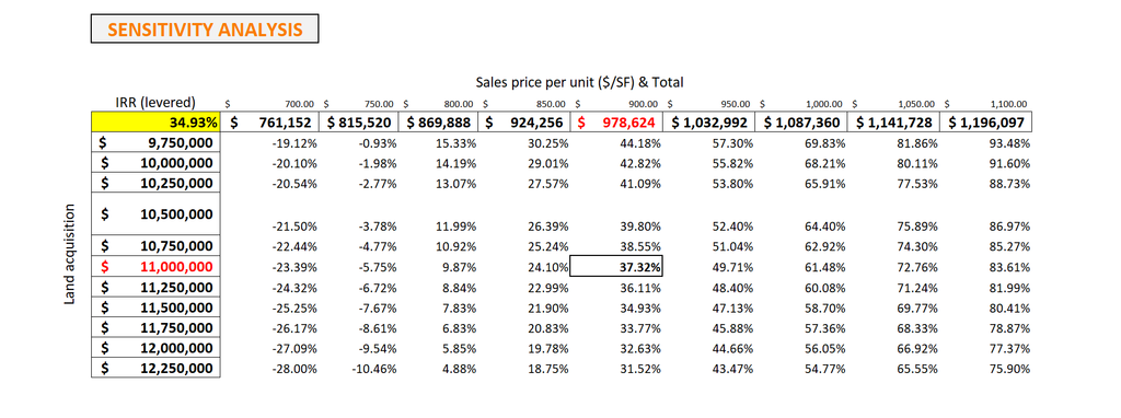
The top two variables from step 4 go on the axes: exit cap rate across the columns and rent growth down the rows. In Excel, use Data, What-If Analysis, Data Table, with the row and column input cells on the same sheet. Link the corner cell to the IRR formula. Shade every cell below the 8.0% hurdle.
Table D. Two-way table: levered IRR by exit cap rate and rent growth
(*) Below the 8.0% preferred return
| Rent growth / Exit cap | 6.50% | 6.75% | 7.00% | 7.25% | 7.50% | 7.75% |
| 4.0% | 17.79% | 16.25% | 14.75% | 13.26% | 11.80% | 10.35% |
| 3.0% | 14.69% | 13.08% | 11.49% | 9.92% | 8.37% | 6.82%* |
| 2.0% | 11.34% | 9.64% | 7.95%* | 6.27%* | 4.59%* | 2.90%* |
| 1.0% | 7.69%* | 5.86%* | 4.02%* | 2.18%* | 0.33%* | -1.56%* |
Every cell in the 1.0% rent growth row falls below the hurdle. At 2.0% rent growth, the deal falls below 8.0% from a 7.00% exit cap onward. At the base case rent growth of 3.0%, a 7.75% exit cap rate removes the preferred return.
Use two variables on the axes, not three. A reader cannot evaluate a three-dimensional grid.
Common error: choosing the axes by habit instead of by the step 4 ranking.
Principle: The range is the analysis.
Step 6. Find the Breakevens
A breakeven is the value at which a target fails. Use Excel’s Goal Seek, or build a table of small steps, to solve for the exact threshold. Report both the threshold value and the distance from the base case.
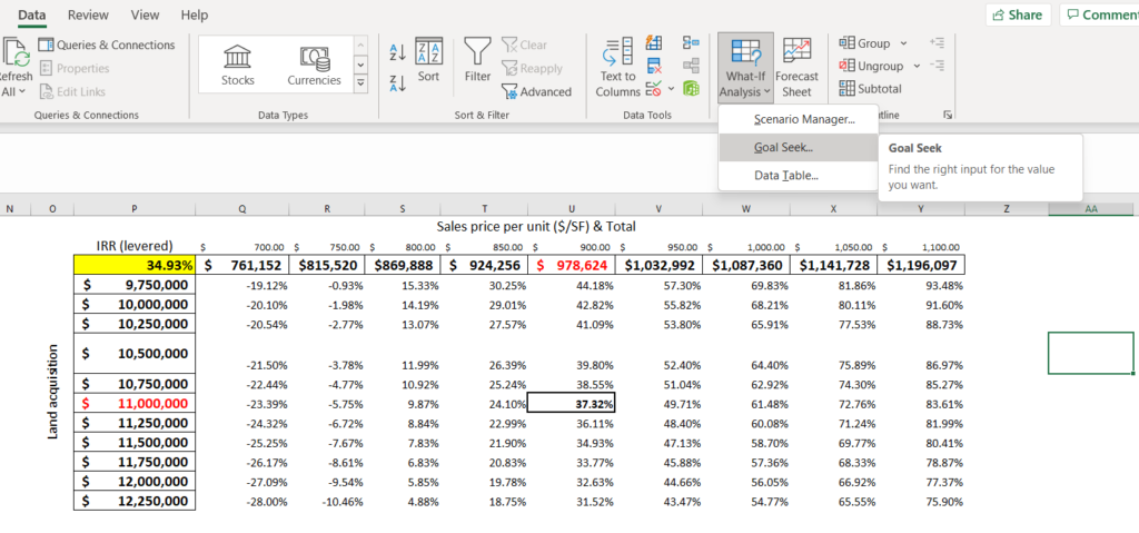
The distance is the number a capital partner needs: not “the deal is sensitive to exit cap rates” but “the deal fails the preferred return after a 56 bps rise.”
Table E. Breakevens
| Question | Answer | Distance from base |
| Exit cap rate at which IRR equals 8.0% | 7.56% | +56 bps |
| Exit cap rate at which equity multiple equals 1.00x | 8.85% | +185 bps |
| Rent growth at which IRR equals 8.0% | 2.01%/year | -0.99 points |
| Rent growth at which equity multiple equals 1.00x | 0.09%/year | -2.91 points |
| Vacancy at which year-1 DSCR equals 1.25x | 25.5% | +18.5 points |
| Vacancy at which year-1 DSCR equals 1.00x | 35.4% | +28.4 points |
The preferred return fails after 56 bps of exit cap expansion. The lender’s coverage test would not bind until vacancy reaches 25.5%, a gap of 18.5 points from the base case. The two audiences face entirely different thresholds from the same deal.
Common error: ending the analysis at sensitivities and never stating the threshold.
Principle: A breakeven answers “how wrong can I be”.
Step 7. Combine Variables and Test Both Views
Variables do not move independently. A demand slowdown raises vacancy and slows rent growth simultaneously. Rising rates push up the exit cap rate and financing cost together. A combined case captures this by changing multiple inputs under one consistent narrative.
Build one downside case that one story can explain. Record IRR, equity multiple, and DSCR together. Then build a severe case to test capital preservation.
Combined cases
| Case | IRR | Equity multiple | Year-1 DSCR | Change in IRR |
| Base | 11.49% | 1.62x | 1.72x | — |
| Downside: exit cap 7.50%, rent growth 2.0%, vacancy 9.0% | 2.40% | 1.11x | 1.67x | -910 bps |
| Severe: downside + rent growth 1.0%, expense growth 4.0% | -3.96% | 0.84x | 1.67x | -1,545 bps |
The downside case shows a DSCR of 1.67x and an equity IRR of 2.4% at the same time. A lender reviewing DSCR sees a deal that holds up. An equity investor reviewing IRR sees a near-zero return on committed capital. Both are reading the same cash flows.
This contrast is the second non-obvious finding in the worked example. It surfaces only when the analysis produces a combined case with both metrics side by side.
Common error: showing only single-variable results and omitting the combined case.
Principle: Variables move together, and the two audiences read different metrics.
How Leverage Changes the Ranking
Leverage amplifies sensitivity to the exit cap rate. The same 50 bps move costs more IRR at higher loan-to-value ratios because debt does not share proportionally in the downside on the equity side.
Table F. Leverage and the exit cap rate: IRR before and after +50 bps
| Loan-to-value | Base IRR | IRR at 7.50% exit cap | Change |
| 0% (unlevered) | 8.07% | 6.86% | -121 bps |
| 50% | 9.97% | 7.68% | -229 bps |
| 65% | 11.49% | 8.37% | -313 bps |
| 75% | 13.38% | 9.25% | -413 bps |
At 65% LTV, a 50 bps exit cap move costs 313 bps of IRR. The same move costs 121 bps on an unlevered basis: about 2.6 times as much. The 25 bps step table below shows the same pattern at finer resolution.
Table G. Exit cap rate steps (65% LTV)
| Exit cap change | Exit cap rate | IRR | Equity multiple | Sale price |
| Base | 7.00% | 11.49% | 1.62x | $26,658,004 |
| +25 bps | 7.25% | 9.92% | 1.52x | $25,738,763 |
| +50 bps | 7.50% | 8.37% | 1.42x | $24,880,804 |
| +75 bps | 7.75% | 6.82% | 1.33x | $24,078,197 |
| +100 bps | 8.00% | 5.27% | 1.25x | $23,325,754 |
Each 25 bps step costs approximately 155 bps of levered IRR in this deal. The same 25 bps step costs roughly 60 bps on an unlevered basis. Leverage raises the return and the sensitivity together.
Sensitivity Analysis in Commercial Real Estate by Property Type
The variables that rank first differ by asset class because income structure differs. The table below synthesizes practitioner patterns, not market research. The editor reviews it against BlueStar Consulting’s direct experience in office, retail, and mixed-use before publication.
| Property type | Variables that usually rank first | Why |
| Multifamily | Rent growth, operating expense growth (insurance and taxes), exit cap rate | Short leases reset rents quickly. Expense growth compounds over a 5-year hold. |
| Office | Lease rollover and downtime, tenant improvement and leasing cost, exit cap rate | Large single-tenant events move cash flow in steps. One tenant at 40% of NOI is a binary risk. |
| Retail | Tenant sales performance, co-tenancy provisions, anchor expiry, vacancy | Percentage rent and anchor loss can restructure the entire income stream. |
| Industrial | Rent mark-to-market at rollover, lease term, exit cap rate | Contract rents often sit above or below market at rollover, so lease timing drives results. |
| Development | Construction cost, lease-up pace, exit cap rate, interest during construction | Cost and timing move the return before stabilization. See the real estate feasibility study guide and the development pro forma. |
How to Present the Results to Capital Partners and Lenders
Lead with one sentence: the base return, the variable the deal depends on, and the breakeven. For this deal: “The base case delivers an 11.49% levered IRR. The return depends most on rent growth and exit cap rate. A 56 bps rise in the exit cap rate removes the 8.0% preferred return.”
Then present the analysis in this order.
| Element | What it shows | Why this order |
| 1. Base case and output metrics | IRR, equity multiple, DSCR, hurdle | Sets the reference before any sensitivity |
| 2. Ranked one-way table | Which assumption the deal depends on most | Tells the reader where to focus |
| 3. Two-way grid with hurdle shading | How the top two variables interact | Shading makes the threshold visible without explanation |
| 4. Breakeven table | How far each assumption can miss before the target fails | Answers the partner’s first question |
| 5. Combined downside with equity and lender metrics | Capital preservation and coverage together | Shows both audiences’ verdicts on the same cash flows |
| 6. Assumptions log with range sources | The evidence behind each range | Lets a partner challenge the ranges rather than dismiss the analysis |
A short narrative accompanies each scenario: one sentence on what conditions it represents and why those conditions are plausible. Document the source for each range. A partner who cannot see where the ranges came from will challenge the analysis rather than engage with it.
One note for passive investors: ask the sponsor for the ranges, the breakevens, and the combined case. A table that shows only favorable-to-base comparisons is not a full analysis.
Avoid building sensitivity tables solely to persuade. Investors in public forums have noted that some syndicators construct charts to support a predetermined conclusion. A credible table shows a case where the deal fails.
Common Mistakes
| Mistake | Effect | Fix |
| Same percentage step for every variable | Ranks variables by how the step was set, not by risk | Set each range from market evidence |
| Flat rent growth in a softening submarket | Overstates every year of income | Test a lower growth case at the submarket level |
| Stabilized vacancy used during lease-up | Understates early vacancy | Model lease-up explicitly and flex its pace |
| Borrowed exit cap rates from another rate environment | Exit value reflects conditions that no longer exist | Anchor on current trades, test +50 and +100 bps |
| Testing only the exit cap rate | Misses the variable that ranks first when ranges differ | Rank at least five variables |
| Optimistic base case | All results start too high | Defend the base case before testing it |
| Ignoring correlation | Understates the downside by separating variables that move together | Build a combined case that one story explains |
| Tables with no interpretation | Readers cannot find the threshold | State the breakeven and the finding in one sentence |
When One-at-a-Time Tests Are Not Enough
A tornado table shows what happens to IRR when each variable moves alone. It cannot show the full distribution of outcomes when many inputs are uncertain and correlated. Monte Carlo simulation addresses this by running hundreds or thousands of scenarios drawn from probability distributions for each variable, producing a range of outcomes rather than a table of discrete cases.
Monte Carlo adds precision, but it requires defensible ranges and explicit assumptions about correlation. The tornado and two-way table are the right starting points for most acquisition analyses.
When a deal has many moving parts, or a decision depends on tail risk, BlueStar Consulting builds both sensitivity work and Monte Carlo analysis as part of custom real estate financial models.
How BlueStar Consulting Approaches DCF Sensitivity Analysis
DCF sensitivity analysis produces cleaner, more defensible results when the base case is built with the same rigor as the stress test. BlueStar Consulting runs sensitivity work on acquisition and development models for investors who already have a model and want an independent check, as well as for clients building from scratch.
The work covers variable selection, defensible ranges, breakeven identification, and presentation-ready outputs for capital partners and lenders.
Already have a model? BlueStar can stress-test it. See real estate financial modeling services or review the real estate investment analysis framework for more context on where sensitivity analysis fits in the broader underwriting process.
Frequently Asked Questions
What is the difference between sensitivity analysis and scenario analysis?
Sensitivity analysis changes one or two inputs while holding all others fixed, then reports how the return metric responds. Scenario analysis changes a set of inputs together under one narrative, such as a recession or an overbuilt submarket. The two tools serve different purposes.
Sensitivity analysis identifies which variable the return depends on most. Scenario analysis tests whether the deal holds up when variables move together. A complete DCF analysis uses both: sensitivity to rank variables, and a combined scenario to test the downside.
Should the discount rate be one of the variables in a real estate DCF sensitivity analysis?
If the output metric is levered IRR, there is no discount rate to flex. The IRR is solved, not discounted. If the output is net present value or property value, flex the discount rate and the exit cap rate together, and avoid counting the same risk twice.
Raising the discount rate to reflect a higher-risk market and also raising the exit cap rate to reflect that same environment double-counts the risk. See the DCF model for real estate for how the discount rate functions in a value calculation versus an IRR calculation.
Why does my Excel data table show the same number in every cell?
The most common causes are: calculation mode set to “Automatic except for Data Tables” in Excel’s formula options, input cells located on a different sheet from the table, or the corner cell not linked to the output formula directly. Check all three before troubleshooting further.
Set calculation to Automatic, move the input cells to the same sheet as the table, and confirm the corner cell references the IRR formula directly. Check current Excel documentation for version-specific steps, as interface locations vary.
Can I build a sensitivity table in Google Sheets?
Google Sheets does not have a built-in what-if data table equivalent to Excel’s Data Table feature. Tables in Sheets typically use array formulas that recalculate the model for each cell, or third-party add-ons.
For complex models, Excel’s native Data Table is more reliable and faster to build. If the team works in Google Sheets, a simplified version can replicate the results with ARRAYFORMULA or by linking individual formula cells manually across the grid.
How often should a sensitivity analysis be updated after closing?
Update the sensitivity analysis at defined triggers: a refinancing, a major lease event, a significant move in market cap rates or interest rates, and before each investor update. Keep the ranges file with the model so the assumptions are traceable.
A sensitivity table built at acquisition and never reviewed may not reflect changed conditions, which matters when a passive investor references it in year three of a five-year hold.
What should an investor do if the deal fails the downside case?
A deal that fails the downside is not necessarily a pass. The question is which variable drives the failure and whether that variable can be addressed. For each driver, there is a corresponding action: renegotiate the purchase price to address an overpriced exit value assumption, reduce leverage to protect against an interest rate move, lengthen the hold period to allow time for rent recovery, add reserves to absorb a vacancy event, or hedge the rate.
A deal that fails under a single variable with an extreme range tells a different story than one that fails under a moderate combined case.